Slitless Grism Spectroscopy
GALEX uses a grism for low resolution slitless spectroscopy. Since GALEX doesn’t have slits, the spectra from objects can, and often will, overlap. The overlaps are disentangled by observing the same field many times with the grism angle rotated relative to the sky. Objects that overlap at one orientation are unlikely to overlap in another orientation. In Figure 1, I show an image in which spectra taken at many grism angles have been added together, yielding “propeller” patterns. There are also no order blocking filters, causing multiple orders to be recorded for each object. In Figure 2, I have plotted image strips (NUV above, FUV below) showing the multiple orders for a very bright blue star. The wavelengths for the 1st, 2nd, and 3rd orders are shown in red, green, and blue, respectively. The second and third FUV orders overlap, which can be a problem for blue objects like the one shown in Figure 2.
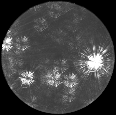
Figure 1. A composite of many individual images taken at different grism angles. The multiple images are used to disentangle overlapping spectra.

Figure 2. Images of spectral strips (FUV below, NUV above) showing the multiple spectroscopic orders. The wavelengths for the 1st, 2nd, and 3rd orders are labeled in red, green, and blue, respectively.
The resolution is roughly 10 Å in the FUV and 25 Å in the NUV. The resolution for resolved objects is worse.
Sensitivity
The sensitivity curves for the FUV and NUV spectroscopy channels are shown in Figure 3. The first, second, and third orders are shown in red, green, and blue respectively. The FUV curves are drawn with dashed lines, while the NUV curves are drawn with solid lines. Note that the most sensitive FUV order is the second. An important thing to remember when considering GALEX’s spectroscopy sensitivity is that every point in the field of view generates a spectrum. Thus, the background level should be constant across the detector and is the integral of the background spectrum across the passbands. Very roughly, the typical level is 1 x 10⁻⁴ (photons s-1 arcsec-2) in the FUV and 1 x 10⁻³ (photons s-1 arcsec-2) in the NUV.
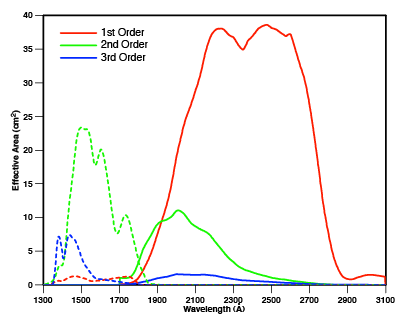
Figure 3. Sensitivity curves for the first three orders (1st red, 2nd green, 3rd blue) for the FUV and NUV channels (dashed and solid, respectively).
In the following two Figures (4 and 5), I show the FUV signal-to-noise ratio per 3.5 Å pixel and the NUV signal-to-noise ratio per 3.5 Å pixel as function of effective exposure time for objects with a wide range of apparent magnitudes. Of course, I leave it up to you, gentle reader, to decide whether a particular signal-to-noise ratio is sufficient for your purposes. When planning observations, remember that the sensitivity falls off radially and that the masking of overlapping objects will reduce the effective exposure time. For high Galactic latitude fields, the typical effective exposure time accounting for the radial response variations and masking is 75 percent of the nominal integration time. One also needs to account for the fact that spectroscopy pipeline only recovers 65 (FUV) to 80 percent (NUV) (with large scatter) of the true flux. I generally find that exposure times needed to achieve a particular signal-to-noise ratio must be three times longer than estimated by the Exposure Time Calculator.
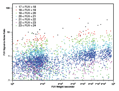
Figure 4. FUV signal-to-noise ratio per 3.5 Å pixel as a function of FUV weight for objects with a range of FUV magnitudes. The FUV weight is the effective exposure time accounting for spatial variations in the detector response and for masking of overlapping neighboring objects.
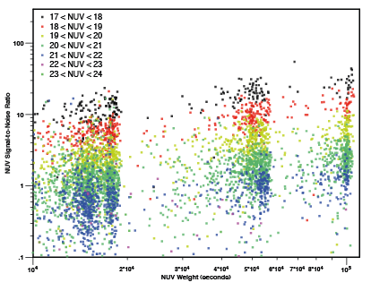
Figure 5. NUV signal-to-noise ratio per 3.5 Å pixel as a function of NUV weight for objects with a range of NUV magnitudes. The NUV weight is the effective exposure time accounting for spatial variations in the detector response and for masking of overlapping neighboring objects.
Data Products
The fundamental product from the spectroscopy pipeline is the image strip. For each sufficiently bright object in a field, one image strip for each band is generated. Each image strip is the analog of the two dimensional spectrum produced by a conventional slit spectrograph, where one dimension is wavelength and the other direction is spatial along the slit. The GALEX image strips contain the first three spectroscopic orders. As I described in the sensitivity section above, the most sensitive orders are 2nd for FUV and 1st for NUV. Because each point in the sky generates a spectrum, the background should not vary significantly across the image strip. (On larger scales, the background does, of course, vary.) The image strips are collected in FITS files, one strip per FITS Header Data Unit (HDU). These very large files are named *-fg-prc.fits and *-ng-prc.fits for FUV and NUV, respectively. The data for each strip consists of two columns, one (”dat”) is the data (number of photons) while other (”rsp”) is the effective response (seconds). The header values “PRI_NC” and “PRI_NR” record the dimensions of the image strips. The data values are stored scaled and can be converted to their true value by applying the zeropoints and scales recorded in the header (”datzero”, “datscale”, “rspzero”, and “rspscale”). In Box 1, I show how to read the ninth (for example) image strip in IDL.
Box 1. IDL code for extracting the image strip for the ninth spectrum in a *-prc.fits file.
The relationship between wavelength in each order and the position in the image strips is nonlinear but well-described by simple polynomial fits. The polynomial fits, whose coefficients are given in Table 1, give the distance (in arcseconds) from the location of the undeviated wavelength as a function of wavelength. The pixel position can then be computed using the scale (keyword “scale” in the *-prc.fits file headers) and the spatial offset of the first pixel from the pixel of the undeviated wavelength (keyword “arcsec1” in the *-prc.fits file headers). As an example, suppose I want to know where on an the FUV image strip with the standard scale 1 arcsecond per pixel and standard first pixel offset of -100 arcseconds light with wavelength of 1550 Å lands in second order. Using the coefficients listed in Table 1, I find that 1550 Å in second order is located +271.1 arcseconds from the position of the undeviated wavelength, which converts, using the 1 arcsecond per pixel scale and -100 arcseconds first pixel offset to pixel 371.
| Order | FUV Polynomial Coefficients | |||
|---|---|---|---|---|
| 1 | -4.288 x 10³ | 6.719 | -3.643 x 10⁻³ | 6.897 x 10⁻⁷ |
| 2 | -4.531 x 10³ | 7.386 | -3.925 x 10⁻³ | 7.475 x 10⁻⁷ |
| 3 | -4.466 x 10³ | 7.484 | -3.863 x 10⁻³ | 7.356 x 10⁻⁷ |
| Order | NUV Polynomial Coefficients | |||
|---|---|---|---|---|
| 1 | -8.821 x 10² | 7.936 x 10⁻¹ | -2.038 x 10⁻⁴ | 2.456 x 10⁻⁸ |
| 2 | -8.142 x 10² | 9.162 x 10⁻¹ | -1.638 x 10⁻⁴ | 1.867 x 10⁻⁸ |
| 3 | -9.182 x 10² | 1.239 | -2.330 x 10⁻⁴ | 2.859 x 10⁻⁸ |
Table 1. Coefficients of polynomial fits to function that translates wavelengths to spatial offsets in the image strips.
The one dimensional spectra are extracted column-by-column by adding up the data in a fixed window of width 15 arcseconds and then subtracting the average of the values in the background windows on either side of the extraction window. The extraction is a simple addition. Optimal weighting (Horne 1986) according to the noise of each pixel is not done (but will be in the future). For a particular object, you may be able to extract a higher signal-to-noise ratio spectrum by subtracting a fit to the background and performing an optimal extraction. All the one dimensional spectra from a field are collected in a FITS binary table, named *-xg-gsp.fits, with each row containing all of the information for each spectrum. There are 58 columns. The IDL code shown in Box 2 will extract, for the i-th spectrum in the file, the wavelength scale, spectrum and error spectrum and convert to Fλ (ergs cm-2 s-1 Å-1).
Box 2. IDL code for reading a one dimensional spectrum and converting it to Fλ (ergs cm-2 s-1 Å-1).
Alas, the image strips are not stored in the same order as the one dimensional spectra in the *-xg-gsp.fits files. To find the image strip corresponding to a particular spectrum in the *-xg-gsp.fits file, you have use to the *-fg-gsax.fits (FUV) and *-ng-gsax.fits (NUV) files as intermediaries. The entries in the *-gsax.fits files are labeled by the spectroscopic ID. The index of the entry with the correct spectroscopic ID will also be the index of the HDU in the corresponding *-prc.fits file where the correct image strip can be found.
Quality Assessment
Through the heroic efforts of several of your GALEX colleagues, every spectrum has been given two quality grades, one for FUV and the other for NUV. There are only three grades:
- It's hopeless to try to extract a useful spectrum.
- There are significant background fluctuations marring the spectrum.
- There are no obvious problems with the spectrum.
The first step in assessing the quality of the spectrum is automated. A program computes the ratio of large-scale background fluctuations to small-scale background fluctuations. The large-scale background fluctuations are estimated simply by measuring the standard deviation of the background spectrum. The small-scale background fluctuations are computed by measuring the standard deviation of the residual fluctuations after subtracting a heavily median-smoothed copy of the background spectrum from itself. If this ratio is above 1.3 for FUV or above 1.5 for NUV, the spectrum is automatically given a grade 1. The human assessors then look to see if there are background problems that were not caught by the automated process and to judge whether, for some reason, there are such large background problems that a meaningful spectrum cannot be extracted. We have worked hard to make the human assessors as consistent as possible, and each spectrum has been examined by at least three people, with the final grade being an average of their grades. Perfection is, of course, impossible to achieve. Therefore, I recommend that you consider the grades as a guide, but not an ironclad one. Most grade 1 spectra still have useful information. You should not, however, use the spectra without first carefully examining the image strips for the object. The grade 0 spectra are generally useless. However, if your favorite object in the universe has received a grade 0, you might still want to look at the image strip and see if there is some information to be salvaged.
There are three particular things that we did not include in our grading. First, we did not mark down a spectrum grade merely because the signal-to-noise ratio was very low. Second, we did not downgrade a spectrum for which the spectral extraction did not recover the full flux of the object (as measured in the direct imaging). The problem of not recovering the full flux is, alas, very common and can be easily identified by comparing the integrated spectroscopy flux with the direct imaging flux. Finally, we did not downgrade spectra with large flux errors at the edges of the two bands. This problem is ubiquitous and is due to the combination of the rapidly falling sensitivity at the edges of the bands and slight wavelength mismatches between the uncalibrated spectrum and the response function.
Gallery
I’ve collected a sample of semi-randomly chosen spectra from the SIRTFFL_00 field to illustrate the quality of the spectra as a function of signal-to-noise ratio. The gallery is on the web here.
GALEXSpec
I have developed an IDL tool for examining large numbers of GALEX spectra efficiently. A screen shot of the main window is shown in Figure 6. The code is not professional quality by any means and is not an officially supported GALEX product (as far as I know -- I’ve been surprised before). However, if you’d like to use the program or, at the very least, have the code as guide for accessing the data with IDL, it can be found here.
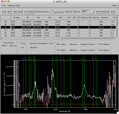
Figure 6. A screen shot of the main window of the GALEXSpec program. The spectrum shown is that of a z = 0.6 quasar.
