


GALEX Frequently Asked Questions
- 101. What are the timing and repeatability issues with GALEX observations?
- 102. What are important factors in estimating the spectroscopic S/N and flux level for an object?
- 103. What are the dead time and gain-sag issues?
- 104. What waivers can be considered?
- 105. Can a GI request an offset of the field center to avoid glints or reflections that scatter into the field of view?
- 106. What unforeseen variables could degrade an observation?
- 107. What observation issues, modes, or special requests will place additional labor burdens on mission planning?
- 108. What are some conditions under which the pipeline might unexpectedly fail?
- 109. How do the low-response regions of the FUV affect off-center objects?
- 110. How may a GI get microsecond timing resolution in phase 2?
- 111. Are imaging observations required for all fields observed spectroscopically?
- 112. What are the ramifications of MPS visibility ratios >5%?
- 113. How well will the spectroscopy pipeline handle extended objects?
- 114. Might proposed observations that are deemed feasible (or resolvable in Phase 2) during the Technical Review be found to be infeasible during Phase 2 planning, after a proposal is selected?
- 115. How can one extrapolate the S/N with exposure time (deep imaging limits)?
- 116. Are there non-standard pipeline products that might be of assistance to some GI programs?
- 117. Should the brightness checker be waived if the field has already been observed by GALEX?
- 118. What is the 'Sky Plot Tool' 'Automated Observation Report'?
- 119. What is the 'Visibility Tool' 'Automated Observation report'?
- 120. Why are the edges of the detectors to be avoided?
- 121. What is the Exposure Time Calculator (ETC)?
- 122. Can I see some example spectra?
- 123. What is the minimum exposure time that can be proposed?
- 124. How accurate is the level of the flux in the grism spectra?
- 125. What are the count rate limits and what is the Petal Pattern mode?
- 126. How do I coadd my new GI observations to preexisting GALEX data to improve S/N (Special Coadds)?
- 127. Why do bright star failures vary between the Brightness Checker and Sky Plot Tools?
- 128. What limits do source confusion place on the depth attainable in deep GALEX exposures?
- 129. What are some common problems with extracting photometry from GALEX images?
- 130. Which of the many flux measurements in the GALEX catalogs should I use?
101. What are the timing and repeatability issues with GALEX observations?
- 101.1 - What are data Drop Outs?
Data dropouts are caused by transmission problems during ground station contact. The effect can be anything from the loss of a few seconds to 100s of seconds in an eclipse. The data loss is taken into account in the tally of total exposure time for an observation. An attempt is made to re-plan the observation if more time is needed to meet the exposure goal. Another attempt to re-transmit the same data may be made, but there is no guarantee that that part of the solid state recorder would not have been over-written with new data by the time the next contingency pass comes around.Although the vast majority of eclipses are returned unaffected by data dropouts, if a proposer is relying on a continuous exposure (a) covering a particular time, or (b) needing to be of a particular length, or (c) needing to fully satisfy a particular sampling strategy, there is some small added risk that the science goals will not be achieved. The risk grows with the length of time or number of samples required.
- 101.2 - What is the observation time precision?
A given sky position cannot be observed at an arbitrary time. Even during the period when the sky position is available, observation times are limited to times the spacecraft is in eclipse and out of the South Atlantic Anomaly (SAA). Thus a series of observations which require highly precise observation times, perhaps to fulfill a specific sampling strategy, may or may not be achievable. The entire GI program must be planned together with the PI observations before specific observation times are known. Small numbers of individual eclipses -- e.g. to catch a target of opportunity -- can be scheduled with an average precision of about 35 minutes (roughly the average time to the next eclipse) when the target is observable. (Details in phase 2, see FAQ 114.)Also note that once a time-critical observation is assigned a given eclipse and the mission planning software sets the start and stop time to the exact second, we only have absolute knowledge of the observation start and end times to between 1 and 10 sec, due to the uncertainty in setting the spacecraft clock. This applies to the photon time tags as well and represents an overall uncertainty in absolute time relative to NIST official time. Also note that the predicted times of eclipses are inaccurate by perhaps a few 10s of seconds when we project a year or so into the future due to limited accuracy in propagating the spacecraft ephemeris.
- 101.3 - What about observation repeatability?
Any or all of these observation characteristics may change from observation to observation for a particular field:
- Field-of-view center and spacecraft roll, and thus where on the detector a given object falls, and thus the detector's uncorrected response
- Detector sensitivity loss due to dead time
- Exposure time
- Radiation environment
- Zodiacal background brightness
- Earth glow brightness
- 101.4 - What is the photon time precision?
Photons are tagged with 5 milliseconds or 20 microseconds precision, depending on the compression mode. (See FAQ 110.) - 101.5 - What are issues with the photon time accuracy?
Analysis requiring accurate photon timing should take into account the global deadtime effects described in FAQ 103, which vary with the global countrate, which in turn varies as stars go in and out of the fov with spacecraft pointing dither. Such analysis will also need to take into account the drift in event timing that is caused by spacecraft clock drift, which is corrected by weekly updates to spacecraft computers. I.e. photon event timing will drift during the week by up to a second.
102. What are important factors in estimating the spectroscopic S/N and flux level for an object?
The actual S/N for a spectra is less than the idealized S/N which would be computed based on the GALEX effective area (see EA curves) and estimated object and background flux. This is due to several factors:
- The flux loss due to a narrow extraction aperture of 10 arcseconds (this depends on the PSF and actual size of a source),
- Low-response areas of the detectors (see FUV flat field image and NUV flat field image),
- Dead-time corrections (effectively reducing the exposure time in the NUV by 10%; see FAQ 103),
- Losses due to masking (ignoring) regions contaminated by neighboring objects (amount of loss depends on the brightness of the object and source density of the field).
In GR2 (2006) and later data releases, the aperture throughput is about 98% (with a PSF of about 5-6 arcseconds), the low response throughput is 75%, the dead time throughput is 90%, masking factor is 85%, and about 99% of visits are accepted (no bad PSFs or other problems). This yields a total throughput (relative to the ideal case) of 56%.
This implies that the actual S/N will be 75% of the ideal estimate. However, the ETC includes these factors, so the estimated S/N from ETC should be approximately correct (see the exposure time calculator (ETC) and FAQ 121).
More information on the spectroscopy sensitivity is given in the GALEX Spectroscopy Primer.
103. What are the dead time and gain-sag issues?
There are essentially two sources of photometric non-linearity in the GALEX instrument: global dead time resulting from the finite time required for the electronics to assemble photon lists, and local sensitivity reduction resulting from the MCP-limited current supply to small regions around a bright sources (gain sag). (The microchannel-plate, or MCP, electron-multiplier array is the central component of the GALEX detectors.)
Global dead time, defined here as the fraction of detected events lost due to the finite processing speed of the electronics, increases monotonically with global input count rate. It is easily measured using an on-board pulser, which electronically stimulates each detector anode with a steady, low rate stream of electronic pulses that are imaged off the field of view. Since the real rate of these pulses is accurately known, the measured rate is used by the pipeline to scale the effective exposure and thus correct the global dead time for all sources in the field simultaneously. This correction is typically about 12% in NUV (for 25 k/sec) and negligible in FUV, however it can become as large as 31% for NUV=80 k/sec, and 8% for FUV=15 k/sec, for the brightest fields that GALEX observes.
The actual fraction of observing time lost is 1-(1/(1+Td*R)), where R is the corrected count rate, which is what is seen in GALEX data products, and Td is a constant, 5.52e-6 sec, which is the (non-paralyzable) deadtime for each photon event. The deadtime correction returns the proper fluxes, but, of course, does not alter the reduced SNR that results from the loss of observing time. To mitigate the effect of deadtime on SNR, one has to increase the actual exposure time on the spacecraft by a factor of 1+Td*R. Note that the GALEX ETC (FAQ 121) was calibrated to be correct for test fields with ~20 k/sec NUV, where the factor 1+Td*R is 11%. Thus, in general, relative to the ETC prediction, the correction factor for NUV is 1+(Td*R)-0.11 and 1+(Td*R)-0.015 for FUV.
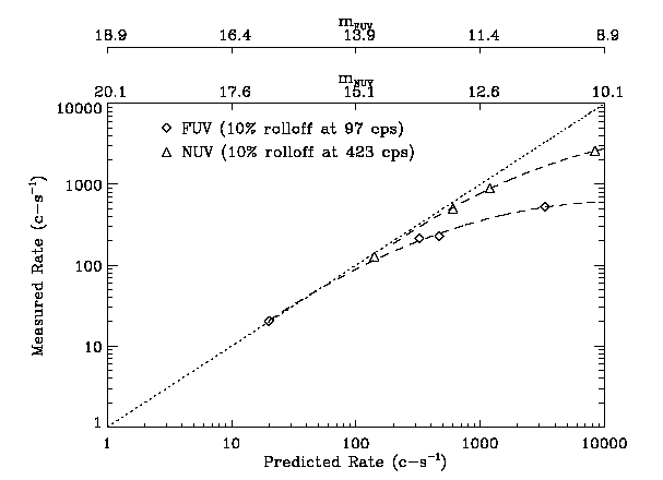
Local dead time, an effect due to the limited ability of MCPs to provide current to a locally-intense region of illumination, is difficult to correct with high accuracy because it requires many observations to calibrate sufficiently and because it is a function of MCP gain, which varies over the detector. It affects not only the measured count rate of individual bright sources but also the source shape. We have used our standard stars to estimate the local dead time in each band as shown in the count-rate linearity figure. Note that because these observations are corrected for global dead time effects, the dead time shown in the figure is zero up to the point where the MCPs begin to suffer from gain sag. The gain sag causes some photon events to fall below electronics pulse-height thresholds. These gain sag effects recover immediately after the bright source is removed (except for very long, bright-source exposures, which we try to avoid because they can eventually fatigue the MCPs, permanently reducing local gain).
The NUV detector is more robust against gain sag from bright sources, because it is proximity-focused and thus presents a larger image (with lower count density) to the MCP. Note that since local photometric non-linearity is strongly source-size dependent, the sensitivity roll off shown in the figure is a worst-case scenario (using stars). See FAQ 125 for a discussion of the current GALEX count rate limits used in planning observations.
104. What waivers can be considered?
- 104.1 Brightness (count rate).
Observations containing a point source with an estimated NUV count rate exceeding 5 k/s will be planned using the petal pattern mode (FAQ 125). A margin of error exists in the count rate limits and a special waiver may be requested if this mode of observations is undesirable.In addition, either the proposer or the science reviewers can request a brightness waiver for a field that violates the count rate limits (local: 5 k/s FUV and 30 k/s NUV; global: 15 k/s FUV and 80 k/s NUV). Granting such requests imposes an additional burden on the mission planners, but the expectation is that modest numbers of moderate violations will be waived. Exact criteria can be developed in the phase-2 technical review after proposals are accepted but before observations are made.
- 104.2 Spacecraft roll angle.
The spacecraft roll angle can be specified for a given observation but requires extra effort by the planning team. This may be allowed for high-value observations if the roll-angle is critical to the science. - 104.3 Zodiacal dark time.
Special scheduling in zodiacal dark times may be allowed however the benefit in almost all cases is minor. GALEX observations can only be scheduled on the night side of the orbit and close to the zenith so Zodiacal background levels are close to minimum for all possible observation periods.
105. Can a GI request an offset of the field center to avoid glints or reflections that scatter into the field of view?
In phase 2, the GI may be allowed to specify an offset to the field center to avoid potential problems with nearby bright objects (depending on the importance of the offset and the personnel time available).
106. What unforeseen variables could degrade an observation?
The PSF may be greatly degraded if there are not enough bright stars in the field to properly align the photon data. This is especially a concern with FUV-only observations.
107. What observation issues, modes, or special requests will place additional labor burdens on mission planning?
Most of the following items require time-intensive manual intervention in the normally-automated mission planning process, and/or add risk that an observation will not be successfully planned due to problems discovered. Associated mission planning risks are listed in parentheses.
- Zodiacal dark time needed--restricts available eclipses (+1)
- A time-critical observation is involved (+1)
- Target of Opportunity (+2)
- Moving target (+2)
- Position proposed as "NA" (unknown) (+1 mps risk)
- A brightness waiver is required (+2)
- Galactic latitude < 10 degrees (+3)
- Galactic latitude < 20 degrees (+1)
- Visibility (MPS) ratio of available to needed eclipses >5% (+1) (FAQ 112)
- Visibility (MPS) ratio of available to needed eclipses >20% (+2)
- Specific grism orientations were requested (+0)
- High photon time resolution (low compression) required
- Other reviewer-determined mission planning issues (+1 to +4)
108. What are some conditions under which the pipeline might unexpectedly fail?
- 108.1 Image reconstruction failure.
In less than 1% of observations, attitude control information from the spacecraft is not sufficient to recover accurate positions and small PSFs. A pipeline step called "deltaphot" uses stars in the field of view to track spacecraft motion more accurately than the spacecraft attitude control system. If presented with an arrangement of stars or spacecraft motion outside its envelope, deltaphot will fail. In most cases, deltaphot can recover good PSFs in such cases, but the astrometry will be poor. In very rare cases, the PSFs are also poor and the data will be very hard to use. - 108.2 Corrupt or missing data.
If a bad ground station contact results in key data being corrupted or missing, the pipeline may be unable to complete. The pipeline is usually robust enough to simply ignore time periods with missing or corrupt data, so most of the time an afflicted observation simply suffers from reduced exposure time. But in unlucky situations, the pipeline can fail outright. This is a rare occurrence.
109. How do the low-response regions of the FUV affect off-center objects?
The FUV sensitivity drops off quickly in two directions away from the center. This drop is large enough (about 30% less response) to significantly effect the actual S/N of an off-center object. See FUV flat field image and compare NUV flat field image. However, the selection of an optimal spacecraft roll angle in phase 2 could mitigate this effect for a given object, but optimal rolls are not always be available.
110. How may a GI get microsecond timing resolution in phase 2?
In phase 2, GIs will be able to specifically request lossless compression mode 1 to gain 20 microsecond photon timing resolution. The standard compression mode 2 allows only 5 millisecond resolution.
111. Are imaging observations required for all fields observed spectroscopically?
Yes, imaging predecessors are required for all spectroscopic observations. In the case of GI spectroscopic observations, this requirement is satisfied if a deep-enough imaging observation of the same field exists or is planned as part of the GALEX surveys. If not, the GI must plan an imaging observation as part of their observing plan. If the GI has not included the imaging predecessor in the proposal, it will be added in the technical review. To be deep enough to satisfy the data-pipeline requirements, the imaging predecessor duration must be at least 5% of the spectroscopic observation duration. Also, new or archival imaging predecessor coordinates offsets must be <1 arcmin or <15 arcmin, respectively, from the new grism observation. As of Cycle 6, any archival image (including from AIS and CAI surveys) may be used as a predecessor, as long as it meets the 5% depth and 15 arcmin offset limits. If the GI must plan an imaging predecessor observation, we will require a minimum of at least 5% of proposed grism exposure time in multiples of 1500 seconds (a typical orbit duration). At the project's discretion, in phase 2 we will make new imaging predecessor observations as short as practical. To GIs performing spectroscopic observations, we will make available all data products for the counterpart imaging predecessors.
The reason for requiring the imaging predecessor is to provide the pipeline with the information necessary to extract spectra to the appropriate sensitivity. All data products will be available to the GI and in the public archive after the GI proprietary period. Though some GIs might prefer to propose shorter-duration observations by eliminating the imaging predecessors, this would eliminate the standard data products and require GIs to extract the spectra themselves. While GIs may be capable of this, the GALEX project has insufficient personnel to answer questions that would likely arise during this special analysis. Also this would eliminate the standard data products from the archive. It is possible that at some time in the future, the spectroscopic pipeline may be upgraded to permit production of standard data products for some fields without imaging predecessors, but this remains speculative at present.
Also note that direct imaging data is highly useful in computing the best possible coordinate system offsets for the grism observations. This means that even if a source RA and Dec position is known, the RA and Dec on the detector must be determined accurately by aligning the grism data with objects (usually stars) of known position and spectra.
112. What are the ramifications of MPS visibility ratios >5%?
If the ratio of ratio of proposed eclipses to viable eclipses for an observation rises above 5%, then the uncertainty in meeting the proposed total exposure time increases (FAQ 107). This is not to say that the proposal is not possible but it becomes increasingly difficult to include such proposals in a mission plan that has to accommodate the successful completion of other plans (GI and PI).
No definite answer can be given during the technical review to any scheduling question, except for the rejection of plans that propose for more eclipses (visits) than are viable for that observation in the during the period of that GI cycle.
The 5% threshold is based on prior experience of the mission planning team, including uncertainty in losses due to detector shutdowns and data transmission dropouts. Eclipses that are lost due to unforeseen circumstances may result in observations not being observed at all during the GI cycle if there is only a narrow range of viable eclipses.
Visibility ratios above 5% translate into a higher risk rating for proposals containing such observations. The risk increases as the ratio increases (FAQ 107).
We also note that the predictions of the orbital motion of the spacecraft during the GI cycle, and hence the eclipse timing, was determined from the two-line element for the GALEX orbit (provided by NORAD) prior to the proposal period. Extrapolating this into the GI cycle observing period adds an uncertainty in the eclipse timing that increases with time. For this reason any proposal that requires a specific date for an observation (the Time-Critical constraint) carries a higher risk of not being scheduled, even if the mission planning system (MPS) data presented in the phase 1 technical review indicates that there are viable eclipses at the proposed observation time.
113. How well will the spectroscopy pipeline handle extended objects?
The spectroscopy pipeline is designed to handle point-source (unresolved) objects. The extraction width or aperture for spectra is fixed at 10 arcsec. Unresolved sources generally have a PSF between 5 and 6 arcsec, resulting in a flux loss of a few percent (see FAQ 102 and FAQ 124). Resolved sources will have a somewhat larger flux loss (e.g. 24% for a source FWHM of 10 arcsec). Large FWHM sources and sources which are broken up into pieces during the direct image source extraction may require a special spectral extraction. Also, non-radially-symmetric sources require special considerations for the grism position angle. A grism image is always provided as a standard product and can be used to extract spectral data by a knowledgeable data analyst. Background subtraction may also be an issue for very wide sources since the sky (background) region begins at 11 arcsec from the center of the source (22 arcsec full width).
Estimating the S/N for an extended object must take into account the larger background area. Note that the loss of spectral resolution should also be considered.
114. Might proposed observations that are deemed feasible (or resolvable in Phase 2) during the Technical Review be found to be infeasible during Phase 2 planning, after a proposal is selected?
There may be some proposals that violate constraints (such as a bright star at the edge of the field of view) which can be resolved with a small amount of planning work (see FAQ 107). These proposals may be recommended for phase 2, however, it is noted that there is still no guarantee that a workable solution will be found. Issues related to scheduling can also be deferred to phase 2.
115. How can one extrapolate the S/N with exposure time (deep imaging limits)?
It is safe to assume that the S/N for a given source will scale as the square root of the exposure time. Note that spatial variations in the detector sensitivity means that the effective exposure time for a given source may vary with parameters such as roll angle between orbits.
Note that the GALEX exposure time calculator (ETC) relies solely upon photon counting statistics to compute the signal-to-noise ratio and does not include the effects of crowding. Due to the rather large GALEX PSF (5" FWHM), crowding in deep exposures is a very acute problem. This may prove to be the limiting factor in the measurement of UV sources with magnitudes ~ 25.
The GALEX science team have been able to reach a depth of at most NUV ~ 25.3 mag using PSF-fitting when relying upon prior information on the positions of sources from higher resolution optical data. This is true even in our deepest fields with exposure times of 240000 seconds in NUV. In principal, crowding is much less severe in the FUV and it may be possible to reach deeper than FUV=25. Deblending of sources in the GALEX EGS observation (237000 seconds NUV exposure) indicates that NUV = 25.3 is the 99% confidence detection limit. See FAQ 128 for more information about source confusion in deep exposures.
116. Are there non-standard pipeline products that might be of assistance to some GI programs?
The pipeline may be run in non-standard ways to produce extra or different products. Time-tagged photon lists are no longer considered non-standard, but are provided to GI's only upon request, through MAST at the same time as the GI's other data. GIs can request other non-standard products, to be generated on a best-effort basis. These may take 6 months or more to produce, thus they may not be available until after the GI proprietary period expires. In evaluating a proposal which promises analytical difficulties, science panel members may wish to ask the PI team whether there are non-standard products which may be of assistance. Keep in mind, however, that whether or not a particular non-standard product is helpful requires case-by-case consideration, and even then there's no way to be sure it will meet the GI's precise needs. Producing them also poses a major personnel burden since the pipeline must be run manually.
117. Should the brightness checker be waived if the field has already been observed by GALEX?
No. Even if a violating field has already been observed with GALEX, there is no automatic waiver for new observations of this field. Here's why:
- Since we cannot not re-point or dither with perfect precision, an over-bright star which didn't cause trouble on prior observations may not be so conveniently excluded subsequently.
- The zodiacal background will change with observation date, so a pointing that stayed under the total field countrate limits once may not do so again.
- The particular location of bright objects (or their reflections) on the detector can increase or decrease the count rate by a factor of ~2, thus just a different roll angle could create a countrate violation where one didn't exist before.
- Transient events (mainly transiting satellites) can cause significant increases in total count rate and could cause a violation where one didn't occur before.
These possibilities (plus uncertainties in our model-derived estimates of NUV and FUV flux as used in the brightness checker) are why we maintain a 25% buffer between the maximum mission planning count rate of 80k/s and the spacecraft count rate protection shutdown limit of 100k/s. Since shutdowns waste observing time, we wish to maintain this buffer whenever possible.
Note that fields, whether observed previously or not, which violate the count rate limits, can have a waiver requested by either the proposer or the science reviewers. Granting such requests imposes an additional burden on the mission planners, but the expectation is that modest numbers of moderate violations will be waived. Exact criteria can be developed in the phase-2 technical review after proposals are accepted but before observations are made (see FAQ 104.1).
118. What is the 'Sky Plot Tool' 'Automated Observation Report'?
This FAQ answer has not been updated from a previous version of the Tool, but is the most detailed description available. See gmkey.txt and example plot gmsample.gif.
119. What is the 'Visibility Tool' 'Automated Observation Report'?
This FAQ answer has not been updated from a previous version of the Tool, but is the most detailed description available. See gmpskey.txt and example plot gmpssample.gif.
120. Why are the edges of the detectors to be avoided?
The outer few arc-minutes of each detector provide lower data quality. Here are the things that make analysis there challenging:
- Detector sensitivity is less-well characterized.
- Electric field-induced spatial non-linearities distort the PSF and produce large position errors.
- Because of dithering, the sensitivity changes very rapidly.
- Reflections from near-field bright stars are very common.
- Localized areas of high detector background ("hot spots," etc.) are numerous, especially in the FUV. Since these areas are masked, this leads to a complex response pattern.
121. What is the Exposure Time Calculator (ETC)?
The GALEX Exposure Time Calculator (ETC) estimates the detected counts and signal-to-noise ratio for a wide set of astronomical objects. The program includes spectral energy distributions for stars (specified by temperature and taken from the Pégase library), white dwarfs (blackbody spectrum specified by temperature), galaxies (Bruzual-Charlot solar metallicity models appropriate for E, Sb, Sbc, Sc, and Im types, augmented by a range of observed composite UV spectra from Steidel and collaborators), and quasars (only a single SED available, which is Randal Telfer's combination of the HST radio-quiet composite spectrum (Telfer et al, ApJ, 565, 773) and the SDSS composite spectrum (Vanden Berk et al, AJ, 122, 549). For a given exposure time and location on the sky, the program estimates the detected counts and signal-to-noise ratio using the user input flux (either apparent magnitude in a broad-band filter or a flux density at a reference observed wavelength), the GALEX effective area curves, and models for background flux from zodiacal light and diffuse galactic light. The user may choose to include Galactic extinction (Cardelli, Clayton, and Mathis law with E(B-V) from the Schlegel et al dust maps) and, for a star-forming galaxy, internal extinction (Calzetti law). For extragalactic objects, the user may also specify a redshift (of course) and a Lyman continuum escape fraction. Absorption from the intergalactic medium is applied to all objects with z > 0, although the absorption is negligible for objects with z < 1. Finally, the user can specify the area subtended by the object (the default is 36 sq arcsec for an unresolved source).
More information on the spectroscopy sensitivity is given in the GALEX Spectroscopy Primer. Proposers should also be aware that results from the ETC were calibrated assuming an 11% NUV detector deadtime correction (see FAQ 103).
- 121.1 Surface brightness.
To use the ETC to estimate the exposure time or SNR for surface brightness measurements, a correction to the flux for the area needs to be included. The ETC assumes a constant flux over an area. As an input magnitude use the magnitude per arcsec^2, which is the magnitude of the total object, plus 2.5*log(area), where area is the effective area for the flux subtended on the sky in square arcseconds. This area also needs to be used as input to the "Area" in the "Area and Milky Way Extinction" box in the advanced option for ETC.
122. Can I see some example spectra?
Yes, below are plots of a 10 spectra from the ELAISS1_00 field. The total exposure time is 84,107 seconds in 69 orbits. Note that the bin size is 3.5 Angstroms per bin, not 5.0 as given in the ETC. To convert, multiply the error per bin shown in the plots by 0.84. Shown are the magnitudes in both bands and the one-sigma error array. For unresolved (point) sources with a typical PSF FWHM of 5 arcseconds, the spectral resolution is approximately 20 and 8 Angstroms in the NUV and FUV, respectively. PostScript here. PDF here.
123. What is the minimum exposure time that can be proposed?
The minimum exposure time that can be proposed is 1500 seconds. This is the typical exposure time for a single orbit. Actual exposure times range from 60 to 1710 seconds in a single orbit but the mission planning system cannot guarantee an exposure time of less than 1500s for any particular observation. Proposers are required to give requested exposure times in multiples of 1500 seconds. Thus an observation that needs 2000 seconds to achieve the S/N required for the science objectives must be assigned 3000 seconds in the mission planning system.
124. How accurate is the level of the flux in the grism spectra?
The extraction aperture for grism extractions is 10 arcsec (full width). In GR2 (2006) and later data releases, the PSF is modeled and a correction is applied so that the level of the spectra is accurate for unresolved sources (within the limits of the photon, calibration, and model errors). No adjustment is made for resolved (non-gaussian PSF) sources, and there will be a significant reduction in the level of the spectra for large sources (greater than about 6 arcseconds). In addition, the spectral calibration error is estimated to be on the order of 5 to 10% in the middle of the grism orders, somewhat larger near the edge of each order.
125. What are the count rate limits and what is the Petal Pattern mode?
The mission planning count rate limits are as follows. For all observations, the global count rate limit is 80 k/s NUV and 15 k/s FUV. For AIS the local count rate limit is 30 k/s NUV and 7 k/s FUV. For all other observations, the local count rate limit is 30 k/s NUV and 5 k/s FUV. For local NUV count rates between 5 k/s and 30 k/s, the Petal Pattern mode must be used. Note that the count rate limits quoted here are the *predicted* rates for the nominal detector response. The actual rates for sources at the detector are generally lower, due to dead time (FAQ 103) and sensitivity variations over the detector (FAQ 109). (The data analysis pipeline corrects for these and other effects in preparing data products.)
We observe objects with 5k/s < NUV < 30 k/s in the Petal mode so as not to cause more local detector fatigue in a given location than takes place during non-Petal-mode observation methods using the 5 k/s count rate limit. For survey types other than the AIS we accomplish this by using the Petal Pattern mode, analogous to the AIS, but with legs, or subvisits, that are mostly overlapping to revisit nearly the same part of the sky. (This is in contrast to the AIS, in which legs overlap minimally in order to tile the sky.)
The Petal Pattern consists of 12 legs, the centers of which lie at 30-degree increments on a circle of 6-arcmin diameter (so each leg is separated by 1.55 arcmin). A Petal mode observation takes an entire eclipse. The exposure time for each leg is up to 120 sec (determined by the length of the eclipse). The roll at each leg varies slightly as determined by the minimum solid-body spacecraft inter-leg motion superimposed upon a continuous dither pattern. The average roll for repeated visits will be planned so that the bright-object positions do not repeat on the detector.
In the case of bright, central, science objects-of-interest, the entire Petal Pattern shall be shifted slightly to move the bright object off the circle that contains the petal centers. In planning observations, we will restrict objects with NUV count rates > 5 k/s to be > 10 arcmin from the center of the field of view for any Petal mode observation. The Petal mode observations will have names consistent with the type of survey (usually Guest Investigator Imaging or Spectroscopic, GII or GIS), independent of the fact that they are observed in Petal mode.
126. How do I coadd my new GI observations to preexisting GALEX data to improve S/N (Special Coadds)?
From cycle 5 onwards proposers may request special co-added data sets, made using the GALEX pipeline software.
Special co-adds may be requested for any data that will be released in GR-6, although the maximum exposure time that can be guaranteed is that currently available in GR-4/5 (as listed in TOAST). Special co-adds will be treated the same way as new observations - they will be proprietary to the proposer for 6 months after the proposer is notified of their availability in MAST, and will become public after that. Special co-adds will not become part of the regular GRs, but will continue to remain available as (publicly released) GI data at MAST. New+archival co-adds will become available to the GI's on the same schedule as the new observations. Special co-adds will have all the same data products as standard co-adds, and will be contained in standard (3840 x 3840 pixels, 1.6 x 1.6 degree) GALEX image. For updates, see: http://galexgi.gsfc.nasa.gov/docs/galex/FAQ/Special_coadds.html#coadds
Several combinations are possible:
- Combine observations from more than one data set at the same location. This could be new observations combined with archival, or two different archival data types (e.g., GI and MIS).
- Combine observations at different pointing centers but covering common regions of the sky. This could be where a GI observation partly overlaps a survey observation, with an object of interest in the common area.
- For deep fields or other very long integrations, co-adds may be requested on a specific time-spacing - e.g. monthly, or weekly.
The effort required to implement a special coadd is only worthwhile if it results in a significant increase in Signal-to-Noise ratio. Thus, requests will not be accepted for combinations where the new co-add exposure time is less 125% of the deepest input coadd. Thus, for example: DIS 14000s + MIS 2000s = coadd 16000s (less than 125% of 14000s) would not be allowed. However, DIS 14000 s + GI4000s = coadd 18000s (more than125% of 14000s) would be acceptable.
Special co-adds should be entered in the ARK proposal form, and should be justified in the "Feasibility" section of the Scientific Justification. When combining new GI observations with archival data (GI or survey data), the new observations should be entered in the ARK proposal form, and the additional data sets should be indicated in the individual observation "Comments" field. When combining different archival data types (MIS with NGS, for example), or combinations of more than one archival GI data set, the longest integration data should be entered as an archival observation, and the shorter integration data should be indicated in the individual observation "Comment" field. Proposers should indicate the center position desired (RA, dec) and indicate the diameter of the science target(s) and/or region of interest.
All GALEX users are, of course, welcome to use public data and their own software to produce their own coadds.
127. Why do bright star failures differ between the Brightness Checker and Sky Plot Tools?
There may be differences between the bright star failures in the Sky Plots (with blue hashed circles), the Brightness Checker output (text table linked from Automated Observation Report). These tools do not use identical inputs. Also, the Sky Plot gif shows only NUV bright stars but the Brightness Checker checks FUV, too. In all cases, the Brightness Checker output should be taken as truth.
128. What limits to do source confusion place on the depth attainable in deep GALEX exposures?
Source confusion is an important concern in deep GALEX images and is the dominant factor limiting the depth attained in deep exposures. The standard GALEX pipeline relies upon the SExtractor program (Bertin & Arnouts 1996, A&AS, 117, 393; http://astromatic.iap.fr/software/sextractor/) to obtain source catalogs for each image. As SExtractor was not designed to work in crowded fields, we recommend that users wanting to obtain photometry for deep fields not rely upon the standard GALEX catalogs. These are the "xd-mcat" files for each tile, or equivalently the PhotoObjAll table in the MAST database (http://galex.stsci.edu). Many of the sources in these catalogs at faint magnitudes will be blends of more than one source. The GALEX exposure time calculator does not take into account the source confusion when determining the photometric errors for a given source flux and exposure time and thus will give erroneously small errors for faint sources in deep exposures.
The best way to obtain reliable flux measurements for sources in deep fields is to use PSF-fitting with prior positions specified by an external optical catalog. In this method, the position of each source is held fixed to the optical position and only the total flux is determined by scaling the PSF to each source. For this method to work, the optical catalog must be sufficiently deep to include all sources that may have UV fluxes. Sources that have spectral energy distributions bluer than a constant in f_nu units (ergs/s/cm^2/Hz), or equivalently colors in the AB system less than zero, are very rare. Thus, the optical catalog should be complete to at least the same depth in AB magnitudes as attainable from the GALEX data.
Among the deepest fields observed thus far is the All-wavelength Extended Groth strip International Survey (AEGIS) field. Based upon the GR3 version of this data with total exposure times of 120 ksec and 240 ksec in the FUV and NUV, respectively, we have produced a catalog of sources using the PSF-fitting with optical priors method. The optical catalog in this case is from the CFHT Legacy Survey which has a depth of ~27.5 mag in the u, g, and r bands. (See Chapter 5a of the GALEX technical documentation for more details: http://www.galex.caltech.edu/researcher/techdoc-ch5a.html). Using the PSF fitting, we are able to reach a 5-sigma limiting magnitude of NUV = 25.5 for sources with no neighbors in the optical catalog within 6 arcsec. Sources that are significantly crowded have larger errors. Sources fainter than this can be detected using this method but the magnitude errors increase and the completeness decreases. The FUV images are less crowded due to the lower density of sources and the slightly smaller PSF. Thus, it should be possible to reach deeper levels in the FUV although this has not been quantified yet.
If a deep optical catalog is not available for the area of sky covered by a deep GALEX pointing, it would be possible to extract photometry using PSF-fitting without fixing the position of each source. This would presumably not be able to reach as deep as with the optical prior method but this would need to be quantified as well.
129. What are some common problems with extracting photometry from GALEX images?
In general, extracting photometry from sources in GALEX images is similar to measuring fluxes of sources in the optical and infrared. However, GALEX data users should note that there are a few differences. Probably the most important difference from optical or infrared images is the extremely low background levels observed in the UV. For high Galactic latitude fields, typical background count rates are ~10^-4 cts/sec/arcsec^2 in the FUV and 10^-3 cts/sec/arcsec^2 in the NUV. These count rates correspond to surface brightnesses in AB mag/arcsec^2 of 28.8 and 27.6 in the FUV and NUV, respectively. This means that AIS exposures, in particular, with exposure times as low as 100 sec, will have average background counts in the FUV and NUV of ~0.01 and ~0.1 cts/arcsec^2, respectively. Statistics such as the median and mode are not useful with so few counts. Some source detection software written for optical or infrared data, such as SExtractor, relies upon these statistics to determine the average sky background. These programs can thus give erroneous results when blindly applied to GALEX images with low exposure times. For this reason we have written our own program to make a background map for each field. These are the "skybg" images included in the standard GALEX data products. These images are accurate to within a few percent and are likely sufficient for most purposes. For very low surface brightness sources, users may wish to remeasure the background around any particular source they are interested in.
As with optical and infrared data, users of GALEX data should be careful when using the standard GALEX pipeline catalogs for large nearby galaxies. These are the "xd-mcat" files included with each tile, or the PhotoObjAll table in the MAST database (http://galex.stsci.edu). Sources that are extended can often be "shredded" into more than one source by SExtractor. This problem is worse in the UV, where galaxies tend to be clumpier and more asymmetric than in the optical. When using the current versions of the GALEX catalogs and especially in the AIS, users interested in using the standard GALEX catalogs for extended sources should be careful to check that their sources are not being broken up into multiple detections. Members of the GALEX science team have formed the GALEX Catalog Team (GCATT) and are working to generate a catalog which would include reliable photometry for galaxies up to one arcmin in diameter. There is a GALEX archival project aimed at extracting photometry for all galaxies larger than one arcmin but this relies upon techniques outside the standard GALEX pipeline. A crossmatch between the standard GALEX pipeline catalogs and the Sloan Digital Sky Survey (SDSS) has been provided via the "Casjobs" service at MAST which can be accessed here: http://galex.stsci.edu/casjobs/. The matching sources between GALEX and the SDSS are given in the "xSDSSDR7" table.
Users of GALEX data should be aware that the sky background in GALEX images is in general not a constant across an individual field, particularly in the FUV. The main contributor to the FUV sky background is UV light from hot stars in the Milky Way disk scattering off dust cirrus. There is structure in the cirrus on a wide a variety of scales. Even at high Galactic latitudes, there are areas of the sky where there is significant cirrus structure in the FUV background. Users interested in faint diffuse light in the FUV, such as in low surface brightness galaxies or in the extended disks of spiral galaxies, should be aware of the potential confusion with the Galactic cirrus. There is a fairly good correlation between the 100 micron emission from the dust and the scattered light in the FUV. Although the scatter is substantial, comparison between the FUV and FIR maps of a given patch of sky can help determine whether the emission is likely cirrus or not.
130. Which of the many flux measurements in the GALEX catalogs should I use?
There are many different measurements of the total flux of sources in GALEX images. The choice of which of these measurements to use depends on the nature of the sources being investigated. The most commonly used total magnitudes would be those listed in the "fuv_mag" and "nuv_mag" columns in both the "xd-mcat" files for each tile, or equivalently the PhotoObjAll table in the MAST database (http://galex.stsci.edu). These two measurements are taken from the SExtractor "mag_auto" measurements and are the total magnitude within an elliptical aperture that is scaled by the radial profile of each object. See Bertin & Arnouts (1996, A&AS, 117, 393) or http://astromatic.iap.fr/software/sextractor/ for more details. Thus, the fuv_mag and nuv_mag columns is generally the most appropriate choice for analyzing sources that are resolved.
On the other hand, for sources known to be unresolved at the GALEX resolution, it would be better to use the "mag_aper" measurements in the catalogs. These are fluxes measured in series of seven circular apertures with radii of 1, 1.5, 2.5, 4, 6, 8.5 and 11.5 pixels. The fluxes measured in these fixed circular apertures must be corrected for the light lost outside the aperture. A table of these aperture corrections is given in Figure 4 of Morrissey et al. (2007, ApJS, 173, 682).
For some applications it can be useful to have the FUV and NUV fluxes measured in exactly the same aperture on the sky in both bands. The columns labeled "fuv_ncat_flux" are the fluxes in the FUV image measured within the NUV mag_auto aperture.

